How to use NetCDF files in a model

NetCDF is a file format for storing multi-dimensional scientific data. More information on NetCDF can be found at Unidata.

This page will walk-through a practical example of using a NetCDF file as input data in a model.

Before we start

NetCDF data is a little more complicated than dealing with other basic file types, such as shapefiles, so this tutorial is aimed at advanced RiskScape users. We expect that you:

• Have been through the How to write basic pipelines and How to write advanced pipelines tutorials already.

• Are proficient using RiskScape and other shell commands.

• Are comfortable working with geospatial data and risk analysis models.

The aim of this tutorial is to give you an understanding of how multi-dimensional NetCDF data can be incorporated into a RiskScape model.

Setup

Click here to download the example project that we will use in this tutorial. Unzip the files into a new directory.

Open a command prompt and cd to the same directory. This is where you will run RiskScape.

Note

To use NetCDF files in RiskScape you first need to enable the NetCDF plugin. Refer to Plugins for instructions on how to enable a RiskScape plugin.

The basics

NetCDF files store multi-dimensional data. You could think of the data as arrays that are indexed by one or more dimensions.

For example, say we had a NetCDF file that contained temperature data that was indexed by geospatial points. This data would have two dimensions: the latitude and the longitude of each point.

NetCDF files are useful for storing data with a time component. If our example NetCDF file contained temperature readings that changed over time, then it would have three dimensions: latitude, longitude, and time.

The actual data that is being stored is called a NetCDF variable. In this example, the variable would be temperature.

NetCDF files can contain many variables. Our example file might have multiple variables if several different readings were recorded at each location and time, e.g. air_pressure, wind_speed, swell_height.

An example file

Let’s look at a very simple NetCDF file: data/simple.nc in your downloaded project directory. Try opening this file. This is what the file looks like if we use ncdump to display its contents:

netcdf simple {
dimensions:
    time = 2 ;
    lat = 2 ;
    lon = 2 ;
variables:
    int time(time) ;
    float lat(lat) ;
    float lon(lon) ;
    string example(time, lat, lon) ;
data:

 time = 1,   // time(0)
    2;  // time(1)

 lat = 10,   // lat(0)
    20;  // lat(1)

 lon = -20,   // lon(0)
    -10;  // lon(1)

 example =
  "t(1) at point(10 -20)",   // example(0,0,0)
    "t(1) at point(10 -10)",  // example(0,0,1)
    "t(1) at point(20 -20)",   // example(0,1,0)
    "t(1) at point(20 -10)",  // example(0,1,1)
    "t(2) at point(10 -20)",   // example(1,0,0)
    "t(2) at point(10 -10)",  // example(1,0,1)
    "t(2) at point(20 -20)",   // example(1,1,0)
    "t(2) at point(20 -10)";  // example(1,1,1)
    }

You can see that the dimensions: section tells us what dimensions are used to index the data: lat/lon spatial dimensions, as well as a time dimension.

The variables: section tells us what data is available in the NetCDF file, as well as what dimensions are used to index that data. The main variable in this case is simply called example, and it has time, lat and lon dimensions.

Think of lat/lon as making up a two-dimensional spatial grid that represents the data. Then imagine there being a stack of these grids, one for each time entry.

Reading a simple NetCDF file

To read NetCDF data into RiskScape we need to setup a bookmark.

When setting up a NetCDF bookmark, we need to tell RiskScape the location of the file, and the variables in it that we want to read. The data held by those variables is then combined into a single RiskScape layer.

Open the simple-project.ini file in your project directory, which has the following contents:

[bookmark simple-netcdf]
location = data/simple.nc
format = netcdf
# layer can be a comma separated list of variables to include
layer = example

[model read-netcdf]
framework = pipeline
source = input('simple-netcdf') as example_data

The read-netcdf is a very simple pipeline that loads the file’s data into RiskScape and then immediately writes the result. Try running the pipeline using the following command:

riskscape -P simple-project.ini model run read-netcdf

This should produce an output file called example_data.csv. Open the file - its contents should look like this:

time,lat,lon,example
1,10.0,-20.0,t(1) at point(10 -20)
2,10.0,-20.0,t(2) at point(10 -20)
1,20.0,-20.0,t(1) at point(20 -20)
2,20.0,-20.0,t(2) at point(20 -20)
1,10.0,-10.0,t(1) at point(10 -10)
2,10.0,-10.0,t(2) at point(10 -10)
1,20.0,-10.0,t(1) at point(20 -10)
2,20.0,-10.0,t(2) at point(20 -10)

This gives you an idea of what the data looks like once it’s read into RiskScape. Note that although we only specified the example variable, the dimensions used to index the variable (time, lat, lon) are also included in the resulting RiskScape layer.

Note

RiskScape lets you include multiple variables from the NetCDF file. The only limitation is that all of the included variables must have the same dimensions.

Reading spatial NetCDF data

We have now successfully read the raw NetCDF data, but to do anything useful with it we want it to be spatial data. We want the RiskScape bookmark to turn the lat/lon coordinates into point geometry.

Take a look at the second bookmark in the simple-project.ini file. It is essentially the same, except that we have added crs-name and set-attribute.geometry to turn the NetCDF data into a spatial layer.

[bookmark simple-netcdf-spatial]
location = data/simple.nc
format = netcdf
layer = example
# We need to specify what CRS the coordinates are in (i.e. the WGS84 lat/lon projection)
crs-name = EPSG:4326
# add a new point geometry attribute to the RiskScape layer
set-attribute.geometry = create_point(lat, lon)

[model read-netcdf-spatial]
framework = pipeline
source = input('simple-netcdf-spatial') as example_data

Note

This is the same way you would turn latitude/longitude coordinates in a CSV file into geometry that RiskScape can use.

Now try running the pipeline that reads the spatial NetCDF bookmark.

riskscape -P simple-project.ini model run read-netcdf-spatial

This time it should produce a GeoPackage output file: example_data.gpkg. Open the file in QGIS. You should see four points visible, but if you open the attribute table you will see two time values present at each point.

Using NetCDF hazard or resource data

You may recall that there are two types of layers in RiskScape: relations and coverages. So far we have been reading the NetCDF data as a relation, but to use it as a hazard-layer or a resource-layer, we will need to turn it into a coverage that we can ‘sample’, or spatially match against.

To turn a relation into a coverage we can use the to_coverage() function.

Because the NetCDF data will typically be point locations, we will want to use a Nearest-neighbour coverage. This allows us to match the closest point in the NetCDF data, even if it doesn’t intersect directly with geometry in our exposure-layer.

An example project

Let’s start with a simple example that uses spatial NetCDF data. We have a set of cities in New Zealand, which is our exposure-layer, and we want to match them up to NetCDF atmospheric data.

We will use NetCDF atmospheric data that was produced by the Community Climate System Model project. In our bookmark we will tell RiskScape to download the NetCDF file directly from this link.

The NetCDF file contains two variables we are interested in: the precipitation flux (pr) and the mean surface air temperature (tas, in Kelvin).

Although this atmospheric data has a time dimension, there is only one time step. This means we can effectively ignore the time dimension and treat it as if there are only lat and lon dimensions.

The bookmark to read the atmospheric data looks like this:

[bookmark atmospheric]
description = A sample file from UniData. Has one time step of precipitation flux, \
  air temperature, and eastward wind.
location = https://archive.unidata.ucar.edu/software/netcdf/examples/sresa1b_ncar_ccsm3-example.nc
format = netcdf
layer = pr, tas
crs-name = EPSG:4326
# convert temperature in Kelvin -> Celsius
set-attribute.tas = tas - 273.15
# longitude values are in the range 0 to 360. Convert them to -180 to 180 range
set-attribute.geom = create_point(lat, if(lon <= 180.0, lon, lon - 360.0))

Note

The last line of the bookmark is a little complicated. It is needed because this dataset has stored the longitude value as 0 <= lon <= 360 whereas the EPSG:4326 projection expects -180 <= lon <= 180.

Sampling a NetCDF coverage

To use the NetCDF atmospheric data in a model, we need to turn it into a nearest neighbour coverage.

To do this, we load our atmospheric bookmark as a relation (i.e. bookmark('atmospheric')), and then use the to_coverage() function to turn this into a coverage. We also need to specify that the coverage is a nearest_neighbour index.

We can then use a sample function (e.g. sample_centroid()) to match our exposure-layer up against the NetCDF coverage.

Putting this all together in a pipeline will look like this:

input($exposure_layer, name: 'exposure')
  ->
# load the atmospheric data as a nearest neighbour coverage
select({
  *,
  to_coverage(
    bookmark('atmospheric'),
    options: {index: 'nearest_neighbour', nearest_neighbour_max_distance: $nn_distance}
  ) as nn_coverage
})
  ->
# sample to find the nearest atmospheric data to our exposure-layer element-at-risk
select({
  exposure,
  sample_centroid(exposure, nn_coverage) as sampled
})
  ->
save('results')

To run this example model pipeline, use the command:

riskscape model run atmospheric

It will produce a results.gpkg file. If you open this file, you will see a tas and pr value have been matched against each NZ city.

Tip

You may notice this model is a bit slow to run. This is because it downloads a copy of the NetCDF file each time it is run. You can speed up the model by downloading the file yourself and updating the bookmark location to be the local/downloaded copy of the file.

Modifying NetCDF data on the fly

Using the bookmark() function is a fairly simple way to load the NetCDF data into the RiskScape pipeline. However, often you will want to modify the NetCDF data before you turn it into a coverage. This will become more apparent later, when we look at NetCDF data that has a time dimension.

Instead of using bookmark() to load the NetCDF relation, we can use the input pipeline step to load the NetCDF data. This means our pipeline can manipulate the NetCDF data before it turns it into a coverage.

The following pipeline essentially does the exact same thing as the atmospheric model we ran previously, however, the pipeline is structured quite differently.

input('atmospheric')
  ->
# turn the atmospheric data into a nearest neighbour coverage
group(select: {
  to_coverage(*,
    options: {index: 'nearest_neighbour', nearest_neighbour_max_distance: $nn_cutoff}
  ) as nn_coverage
})
  ->
# join this coverage to our exposure-layer
exposures_atmospheric_join.rhs


input($exposure_layer, name: 'exposure')
  ->
join(on:true) as exposures_atmospheric_join
  ->
# sample to find the nearest atmospheric data to our exposure-layer element-at-risk
select({
  exposure,
  sample_centroid(exposure, nn_coverage) as sampled
})
  ->
save('results')

We still use the to_coverage() function to turn the NetCDF relation into a coverage. However, we now call to_coverage() from a group step.

The other difference is we now need to use a join step to join the two pipeline relations together. We end up with a single nn_coverage attribute on the right-hand-side of the join, and the on: true condition adds this to every row of data in our exposure layer.

To run this example model pipeline, use the command:

riskscape model run atmospheric-join

The results produced should be exactly the same as the atmospheric model you ran previously.

Nearest neighbour triangulation

The atmospheric temperature data in this model uses a coarse resolution grid, which is shown as orange points in the following image:

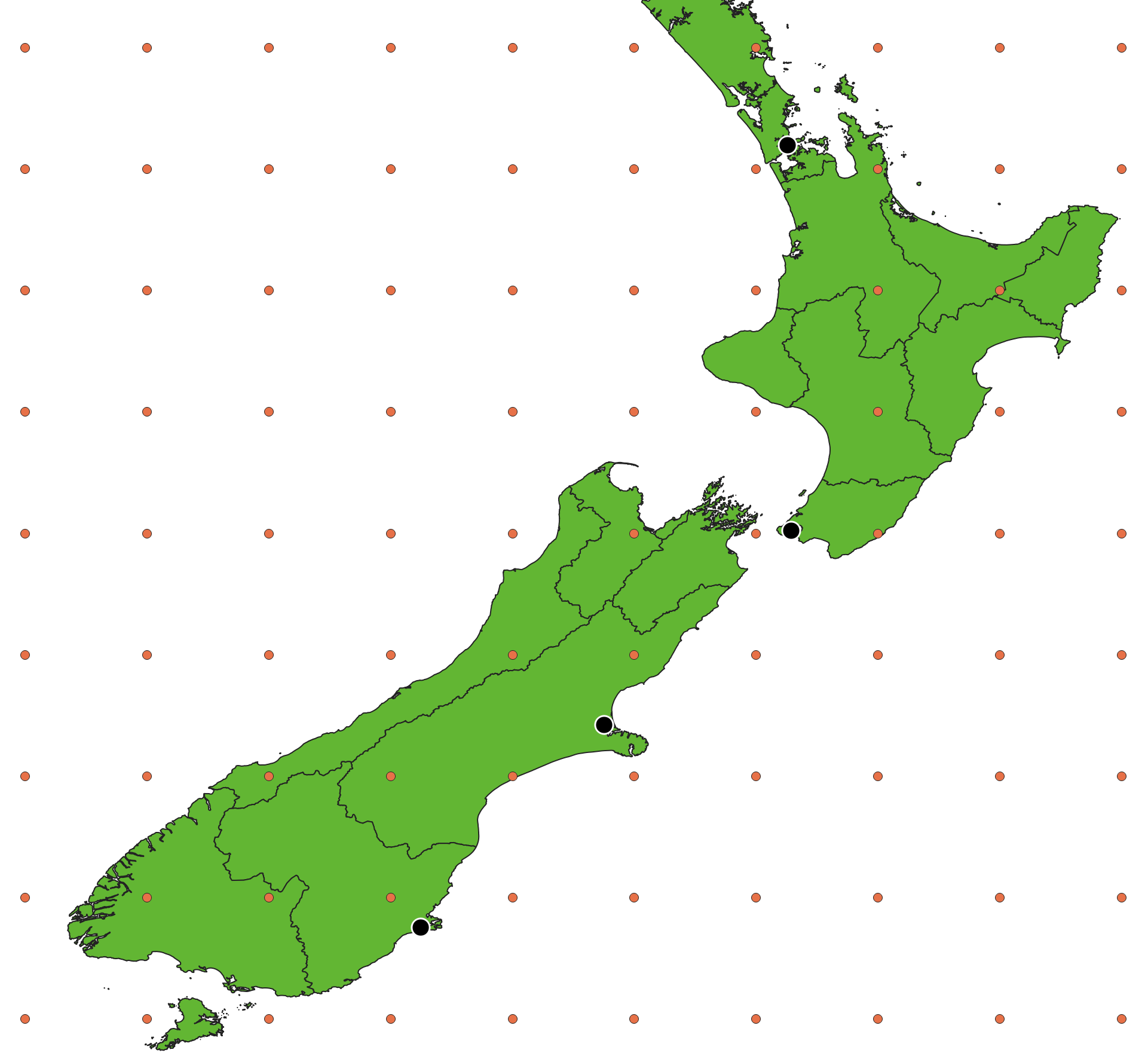
So far, we have been spatially matching our cities (the black points) to the closest temperature reading. An alternative approach is to derive a temperature reading using triangulation. This involves finding the three nearest temperature readings, which typically form a triangle around the city’s location, and then weighting the temperature readings based on how close the city’s location is to each point in the triangle. The technical name for this process is barycentric interpolation, but effectively it is calculating a weighted average of the temperature readings, based on their proximity.

Note

The triangulation feature requires the Beta plugin and may change in future releases.

Again, we can modify the previous atmospheric pipeline to triangulate the sampled data, like this:

select({
  *,
  # Apply a mapping to values from the coverage so that the samples include only the `tas`
  # value - this makes it simpler to use with the triangulate method below, as it expects
  # single numeric value
  map_coverage(nn_coverage, val -> val.tas) as nn_coverage
})
  ->
# sample the 3 closest values to our element-at-risk
select({
  exposure,
  sample_n_closest(exposure, nn_coverage, 3) as samples
})
->
# Triangulate them based on the element's location.  `triangulate` uses barycentric
# coordinate maths to weight the values from the 3 samples 'fairly'
select({
  exposure,
  triangulate(exposure, samples) as triangulated
})

You can run this example and compare the result to our previous runs to see how triangulation affects the sampled results:

riskscape --beta model run atmospheric-triangulated

It should produce a results-table.csv file that looks like this:

name	sample_1	sample_2	sample_3	triangulated	closest
Auckland	14.609	15.222	16.599	15.165	14.609
Christchurch	9.417	9.057	7.919	8.893	9.417
Dunedin	7.253	8.263	8.513	7.816	7.253
Wellington	11.07	11.737	11.713	11.276	11.07

This shows the three nearest temperature readings that were spatially sampled, and the triangulated value, after the barycentric interpolation has been applied. The closest temperature reading, which was used in the previous models, has also been included for comparison, although this is the same as the first sampled value (i.e. sample_1).

Note

The pipeline code shown above does not include the extra sample_N and closest attributes shown in the results. They were omitted from the pipeline snippet for clarity, but you can refer to the atmospheric-pipeline-interpolation.txt file to see the full pipeline code used in the model.

One thing to note about the triangulation in this model is the interplay between the nearest neighbour cut-off distance (i.e. the nn_cutoff parameter) and the sample_n_closest method. If the cutoff distance is too small, you may not get enough samples back to perform triangulation. If this happens, the triangulate method will apply distance-weighted averaging to the two available data-points, or return the singular value if only one data-point was found.

The previous models used a 120km nn_cutoff distance, optimized to make sure centroid sampling always picks up a single point. However, for this model we have doubled that distance by default and use a 240km cut-off to make sure we always pick up the three nearest points.

Try running the following command, which uses the smaller 120km nn_cutoff, and look at the results again.

riskscape --beta model run atmospheric-interpolation -p nn_cutoff=120000

This time, with the smaller cutoff distance for the index, there are fewer samples for each city:

name	sample_1	sample_2	sample_3	triangulated	closest
Auckland	14.609	15.222		14.768	14.609
Christchurch	9.417	9.057		9.264	9.417
Dunedin	7.253			7.253	7.253
Wellington	11.07	11.737		11.261	11.07

In this case, the triangulation will use an inverse distance-weighted average for the two temperature measurements it has available. With three samples, if the element-at-risk falls outside of the triangle (i.e. if a non-uniform grid is used), then the triangulation method would also use only use the two closest data-points in an distance-weighted average. In the case of Dunedin, only one temperature measurement falls within the cut-off distance, so that value is used as is.

Note

Barycentric interpolation and Inverse Distance-Weighting (IDW) are slightly different. IDW simply applies a 1 / distance weighting, whereas with barycentric interpolation the weighting is actually based on areas of sub-triangles formed between the given location and each edge of the triangle.

Using the time dimension in your model

Usually NetCDF data will also have a time dimension, which makes manipulating the data slightly more complicated.

Open your project.ini file and look at the sea-temperature bookmark. This uses a NetCDF file produced by PCMDI, which records monthly sea temperature data for 24 months from January 2001.

Instead of matching a single temperature reading against each of our cities, we now have 24 readings. Our model has to take the raw NetCDF data and group it together in a way that our model can sensibly access.

The simplest approach is to group the raw NetCDF data by geospatial point. Instead of matching each city against a single temperature reading, there is now a list of 24 temperature readings at that point. We can turn rows of data into a list using the to_list() function.

The following example pipeline matches the sea temperate NetCDF data to our cities:

input('sea-temperature')
  ->
# group the sea temperature readings by their spatial location (geom) so that
# we end up with a list of readings. Each list item corresponds to a time entry
group(by: geom,
      select: {
        geom,
        to_list(*) as readings
})
  ->
# now turn the readings into a coverage that we can sample
group(select: {
  to_coverage(*,
    options: {index: 'nearest_neighbour', nearest_neighbour_max_distance: $nn_cutoff}
  ) as nn_coverage
})
  ->
# join the coverage to the exposure-layer
exposure_and_sea_temp.rhs


input($exposure_layer, name: 'exposure')
  ->
join(on: true) as exposure_and_sea_temp
  ->
select({
  exposure,
  sample_centroid(exposure, nn_coverage).readings as readings
})
  ->
unnest(readings)
  ->
save('results')

This pipeline is very similar to the atmospheric-join pipeline in the previous section, except:

• There’s a new second step that uses to_list(). For each point location, this turns 24 rows of temperature reading data into one list with 24 items.

• There’s a new unnest step after we geospatially match the temperature data to our cities. This expands the list again, turning 24 list items into 24 rows of data for each of our cities.

Try running this example using the command:

riskscape model run sea-temperature

Open the results.gpkg file that was produced and check the data. Note that the time values in this data records the days since 1 January 2001.

Aggregating across time

Condensing the NetCDF time dimension into a list can be useful if you are interested in every value across all time steps. However, if you are only interested in the maximum or average value across all time steps, then using a list is actually unnecessary.

Instead of using the to_list() function, it can be simpler to aggregate directly to the value(s) you are interested in. For example:

group(by: geom,
      select: {
        geom,
        min(tos) as min_tos,
        max(tos) as max_tos,
        mean(tos) as mean_tos
})

This approach also makes the unnest step unnecessary. A full example pipeline is available in the sea-temperature-aggregated-pipeline.txt file in your project.

Try running this pipeline using:

riskscape model run sea-temperature-aggregated

Notice that the output is much simpler in that the 24 time steps have now been condensed down into a single row of aggregated values for each city.

Using the pivot feature

An alternative to aggregating the data in the pipeline is to use the pivot bookmark feature.

Remember that NetCDF data is stored in a compact, multi-dimensional grid. Pivoting restructures the data by “unfolding” one of those dimensions into a flat list. Instead of RiskScape treating each item in the specified dimension as a separate row of data, it becomes an item in a list — with the corresponding NetCDF variable data sitting right alongside it.

Our NetCDF dataset here has three dimensions (lat, lon, and time), along with one variable (the tos temperature reading) for each unique combination of dimensions. In the previous example, rows were coming out of the NetCDF bookmark like this:

lat	lon	time	tos
105	88.5	1	271.45
105	88.5	2	271.55
105	88.5	3	271.56
		…
106	88.5	1	271.42
106	88.5	2	271.44

However, if we pivot on the time dimension, then each row of data would now contain a list, consisting of:

• The time value (the dimension we pivoted on)

• The tos value (the sea temperature variable associated with that point in time)

The data produced by the bookmark would look more like this:

lat	lon	readings
105	88.5	[{time: 1, tos: 271.45}, ...]
106	88.5	[{time: 1, tos: 271.42}, ...]

Pivoting on time is effectively the same as aggregating by the other dimensions (lat and lon), which we did in the pipeline in the previous example. A bookmark to pivot on the time dimension would look like this:

[bookmark sea-temperature-pivot]
...
# return time / tos pairs in a list
pivot = time as readings
...

Note that the pivot line in the bookmark specifies an alias for the list of time and tos pairs, so they appear as a readings attribute in the pipeline data. See the sea-temperature-pivot bookmark and models in the projects for a worked example.

Scaling to large datasets

So far our example NetCDF files have been fairly small. The example pipelines so far may struggle to run over very large NetCDF files, due to memory and performance issues.

The pipelines we have been using need to load all the NetCDF data into RAM simultaneously. This may be a problem if the NetCDF file holds several gigabytes of data, such as hazard data for a probabilistic model.

In order to avoid these scalability problems, we want to flip our pipeline on its head: instead of turning our hazard-layer into a coverage, we want to essentially turn our exposure-layer into a coverage.

Whenever we use a join step, we want the right-hand side (rhs) of the join to be the smaller of the two datasets. If our hazard-layer dataset is much bigger than our exposure-layer, then we will want the exposure-layer to be on the right-hand side of the join.

There is a scalable-netcdf model you can try running. It will produce the same results as the sea-temperature model, but it looks up the closest element-at-risk using an exposure-layer coverage this time.

The full pipeline is available in scalable-netcdf-pipeline.txt for you to look at further. A brief overview of what it does:

• We need a separate bookmark that only loads the NetCDF site-mesh, i.e. just the lat/lon dimensions.

• We turn this site-mesh data into a coverage, so that we can match every element-at-risk to the closest lat/lon point in the NetCDF data.

• Using to_list() aggregation will give us a list of elements-at-risk for each site-mesh point.

• We can then go through the NetCDF data one row of data at a time, and match each row against the elements-at-risk it affects, based on the site-mesh point.

• Because we know the exposure-layer will now contain a site-mesh point that exactly matches a point in our NetCDF data, we can look for an exact match in the join step’s on: condition. (Normally, we would need to sample the coverage after the join, but we’ve done the sampling before the join in this case)

Recap

We have delved deep into some advanced pipeline concepts here, so here is a recap of the key points:

• NetCDF files hold multi-dimensional data, usually involving a time dimension as well as geospatial dimensions.

• You need the optional NetCDF RiskScape plugin installed in order to use NetCDF files in your model pipelines.

• RiskScape loads NetCDF data as a relation. The to_coverage() function will turn a relation into a coverage that can be geospatially sampled easily.

• When hazard data is point-based, such as based on a site-mesh, you will likely want to use a nearest neighbour coverage.

• Aggregating across the time dimension makes the NetCDF data simpler for your model to process. You can either aggregate to a list of all values for an element-at-risk over time, or take the max/mean/etc values for that element-at-risk.

• A coverage needs to hold all the data it contains in memory at once. For very large hazard datasets, it’s best to ‘flip’ your pipeline so you essentially turn your smaller exposure-layer dataset into the coverage.