DEVORA case study
This page walks through a worked example of infrastructure risk models for a volcanic eruption. The hazard data used in this example is the ‘Scenario C’ Māngere Bridge eruption, produced as part of the Determining Volcanic Risk in Auckland (DEVORA) research programme.
Tip
This page is aimed at advanced users who are comfortable writing pipeline code. If pipeline code is new to you, try looking at How to write basic pipelines and How to write advanced pipelines first.
The models on this page have been built for demonstrative purposes, and combine the DEVORA hazard data with exposure datasets from Transpower New Zealand’s Open Data portal and Toitū Te Whenua Land Information New Zealand (LINZ). Note that:
The Transpower data is publicly available under the Creative Commons Attribution 4.0 International License (CC-BY 4.0).
The LINZ road and rail data is licensed under Creative Commons 4.0 Creative Commons Attribution 4.0 International.
The hazard data and risk functions used in these models have been provided by the New Zealand Institute for Earth Science Limited (Earth Sciences New Zealand) and are licensed under Creative Commons Attribution-NonCommercial 4.0 International.
Eruption hazard data
This scenario was designed by scientists and emergency managers to simulate a hypothetical eruption within the wider Auckland metropolitan area. The hazard data represents a complex eruption within the Auckland Volcanic Field, which spans 32 days.
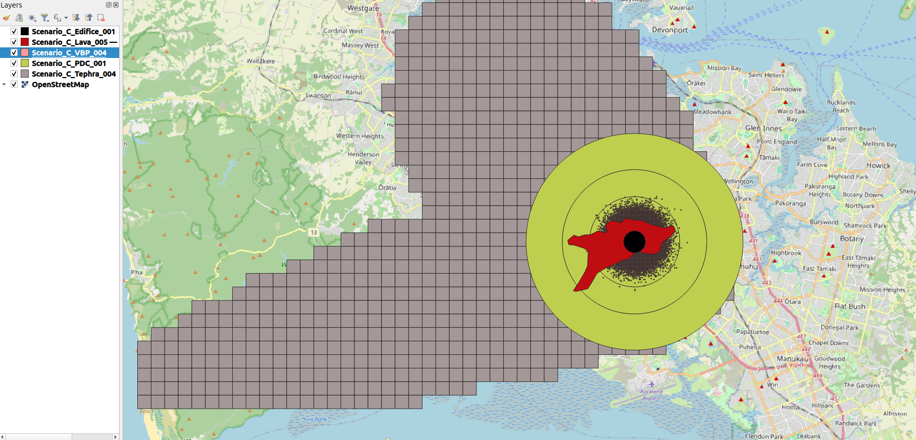
The hazards include ashfall (tephra), volcanic ballistic projectiles (VBP), pyroclastic density currents (PDC), lava, and the body (edifice) of the newly-formed volcano itself. You can learn about the modelled eruption in more detail from the following sources:
Investigating the consequences of urban volcanism using a scenario approach I: Development and application of a hypothetical eruption in the Auckland Volcanic Field, New Zealand (Journal of Volcanology and Geothermal Research)
Economics of Resilient Infrastructure Auckland Volcanic Field Scenario (Research Report)
The simulated eruption occurs over several weeks, with the following notable events producing new hazard layers:
Timeline |
Hazards produced |
|---|---|
March 14th |
Edifice, pyroclastic surge (worst case), ballistics, ash |
March 21st |
Ash, pyroclastic surge (average), ballistics |
March 22nd |
Ash, ballistics |
March 25th-30th |
Ash, ballistics |
April 3rd-14th |
Lava |
The hazard data is cumulative. As the timeline progresses, the hazard data for a given date will also include the hazard footprint for all previous dates in the eruption. So for example, there are four tephra hazard maps - the fourth map corresponds to March 25th-30th and includes any ash that was deposited on previous days of the eruption, i.e. it is a snapshot of what the total accumulated ashfall would look like at that point in time, assuming there is no cleanup between events.
Note that there is only one PDC hazard map, because the pyroclastic surge on March 21st is smaller than the March 14th event, and so it doesn’t increase the hazard footprint at all. The PDC hazard-layer is used throughout the eruption sequence, even though PDC is only produced for the first two dates in the eruption sequence. This is because the model is outputting the cumulative impact of the eruption - so the results for April 3rd-14th will include the impact from PDC on March 14th.
The following is a screenshot of the geospatial hazard data overlaid on an OpenStreetMap background of Auckland.
Case-study project
The files for this RiskScape project can be viewed here.
The best approach to run these models locally is to download (or clone) the whole GitHub repository. You can click on the ‘Code’ button to download the repository as a zip file.
Once the files have been downloaded and extracted on your computer, open a command terminal
and change directories (i.e. cd in terminal) to the case-studies\DEVORA sub-directory.
This directory contains all the hazard data files needed.
The exposure-layers use open-data that can be accessed remotely, via the project’s bookmarks.
Reading the hazard data
The hazard data here spans multiple files in two different ways:
There are five different time periods in the eruption sequence that are being modelled (March 14th, March 21st, March 22nd, March 25th-30th, April 3rd-14th). Each newly produced hazard has been modelled in a separate GeoPackage file.
There are five different hazard types (tephra, VBP, PDC, lava, and edifice). Each hazard type has been modelled in a separate GeoPackage file.
In order to load the hazard data into the RiskScape model, we will use the following approaches:
To process several different time sequences in the same model, we will use the Multi-file hazard data approach. The different hazard time steps are defined in a CSV file that RiskScape then uses to load the hazard data dynamically.
To process several different hazard types at the same time, we will use the Combining multiple hazard-layers approach. This uses the
combine_coverages()function to treat the five different hazard types as a single layer for spatial sampling operations. In other words, we can sample a single combined coverage to determine whether a element-at-risk was exposed to any of the five different hazard types.
Tip
Have a read of the above documentation links for a more detailed explanation of how these RiskScape modelling approaches work. This page will focus on applying these approaches to a model pipeline for the DEVORA case study data.
Hazard CSV file format
The model pipeline accepts a $scenario model parameter, which is a CSV file that contains all the details
of the eruption sequence. This includes the filepath of each volcanic hazard type, for each time-step in the eruption.
By default, the Scenario-C.csv file is used.
The pipeline code to load a CSV file is very simple:
# input the eruption scenario hazard data
input($scenario)
Tip
The $scenario model parameter has been used here to make the model pipeline reusable for modelling other eruptions.
A different CSV file could be used to represent a different eruption sequence for another volcano, providing it
uses the same CSV column names.
The following table shows the first two rows of the Scenario-C.csv, which represent the first two dates in the eruption timeline.
The filenames have been shortened for simplicity.
Note that the tephra and VBP hazard files have been updated in the second row, which incorporates the new hazards
produced by the second eruption event in the sequence.
Timeline |
edifice |
|
tephra |
|
lava |
|---|---|---|---|---|---|
March 14th |
|
|
|
|
|
March 21st |
|
|
|
|
|
Note
In the Multi-file hazard data example, only one hazard file is used per CSV row. Whereas this scenario deals with five volcano hazard types, so five different hazard files are used per row.
Creating hazard coverages
By default, RiskScape will load the filepaths in the Scenario-C.csv as text-string data.
So the model pipeline needs to turn the hazard filepaths read from Scenario-C.csv from text-strings into a ‘coverage’ that can be spatially queried.
To do that, bookmark() will load the vector data dynamically, and then to_coverage() will turn the vector data into a geospatial coverage.
Placeholder bookmarks are used so that RiskScape will know the vector attributes that are present in each GeoPackage file, even though the GeoPackage files are being loaded dynamically. A separate placeholder bookmark is needed for each hazard type: Edifice, PDC, Tephra, Lava, and VBP. The pipeline code looks like this:
# input the eruption scenario hazard data
input($scenario)
 ->
# use placeholder bookmarks to load the hazard filepaths read in from the CSV input.
# The hazards are vector data, so we turn them into a 'coverage' that we can spatially sample
select({
         *,
         edifice: to_coverage(bookmark('Edifice', {location: edifice})),
         PDC: to_coverage(bookmark('PDC', {location: pdc})),
         tephra: to_coverage(bookmark('Tephra', {location: tephra})),
         lava: to_coverage(bookmark('Lava', {location: lava})),
         VBP: to_coverage(bookmark('VBP', {location: vbp}))
})
Combining hazard coverages
We then use the combine_coverages() function to combine these five coverages into
a single coverage, which simplifies the spatial sampling we need to do.
Instead of sampling five different coverages and combining the results,
we can just sample a single combined coverage.
The following RiskScape expression will take the original coverages and combine them into a single coverage (called ‘hazard’).
combine_coverages({edifice, PDC, tephra, VBP, lava}, $grid_resolution) as hazard
When sampling the combined coverage, the name of the original coverage is prefixed to
the attributes in that vector layer. Note that the placeholder bookmarks change the attribute
name to HIM (hazard intensity measure) for each hazard type, because that is the
attribute name that the volcanic risk functions will use.
The following table shows how the attribute name changes as it progresses from the original input file, through the RiskScape placeholder bookmark, through to the final end result returned by a spatial sampling operation on the combined coverage. The final sampled result will be passed to the risk function.
File |
Original attribute |
Bookmark attribute |
Coverage name |
Sampled result |
|---|---|---|---|---|
|
|
|
|
|
|
|
|
|
|
|
|
|
|
|
|
|
|
|
|
|
|
|
|
|
Joining the exposure data
We also need to join the combined coverages to the exposure-layer. This lets us spatially determine whether each element-at-risk in the exposure-layer is exposed to any of the volcanic hazard-layers.
The pipeline code to load the input data for the exposure- and hazard-layers would then then look like this:
# input the exposure layer
input($exposures, name: 'exposure')
 ->
# add in the hazard event data
join(on: true) as join_exposures_and_hazards

# input the eruption scenario hazard data
input($scenario)
 ->
# use placeholder bookmarks to load the hazard filepaths read in from the CSV input.
# The hazards are vector data, so we turn them into a 'coverage' that we can spatially sample
select({
         *,
         edifice: to_coverage(bookmark('Edifice', {location: edifice})),
         PDC: to_coverage(bookmark('PDC', {location: pdc})),
         tephra: to_coverage(bookmark('Tephra', {location: tephra})),
         lava: to_coverage(bookmark('Lava', {location: lava})),
         VBP: to_coverage(bookmark('VBP', {location: vbp}))
})
 ->
# combine the coverages so we can sample a single 'combined' hazard layer in one go
select({
         {
           time_sequence,
           timeline,
           description
         } as event,
         # note that sampling the combined coverage will prefix the sampled attributes with the
         # coverage's name below. So the 'HIM' attribute in the 'tephra' layer will become 'tephra_HIM'
         combine_coverages({ tephra, edifice, pdc, tephra, vbp, lava }, $grid_resolution) as hazard
      })
 ->
join_exposures_and_hazards.rhs
This pipeline code is located in a
sub-pipeline file called hazard-scenario.txt.
Tip
Sub-pipelines allow you to reuse parts of a model pipeline in other models.
So you could reuse the hazard-scenario.txt sub-pipeline to load volcano hazard data
(that’s in the same format) into another model pipeline.
Note
The join condition used here is on: true which means every row of data on the right-hand side (i.e. the hazard data)
is joined to each row of exposure data. This means any given asset will be duplicated five times,
i.e. once for each time-step in the eruption sequence. The model pipeline will then aggregate the results
later to remove the duplication.
Volcanic risk functions
The GitHub repository contains volcanic risk functions for infrastructure that have been provided by Earth Sciences New Zealand under the Creative Commons Attribution-NonCommercial 4.0 International license.
The Python source code for these risk functions can be accessed here. You can refer to the following journal articles for more details about these risk functions:
Improving volcanic ash fragility functions through laboratory studies: example of surface transportation networks (Journal of Applied Volcanology)
Framework for developing volcanic fragility and vulnerability functions for critical infrastructure (Journal of Applied Volcanology)
Volcanic hazard impacts to critical infrastructure: A review (Journal of Volcanology and Geothermal Research)
Calling the risk function
For each event in the eruption sequence, the model pipeline will spatially sample the combined hazard coverage for each element-at-risk. The following data, or ‘function arguments’ are passed from the RiskScape pipeline to the Python risk function:
Exposure: The asset or element-at-risk being modelled. This information is not actually used by the Python code currently. Separate Python code is used for each different category of infrastructure (i.e. roads, railway lines, transmission lines, sub-stations, etc), and the same risk curve is used for any assets in that category.
Multi-hazard: a Python dictionary containing a hazard intensity measure (HIM) for each of the volcanic hazard-layers. This contains the hazard values that were spatially sampled for this particular asset and event from the combined coverage in the RiskScape pipeline.
Random-seed: Optionally seed the random number generation for this particular asset. This controls how the randomness of the function behaves across events for a given asset.
Note
The input data contains a volcanic ballistic projectile (VBP) layer, however, these risk functions do not support a VBP hazard. Currently the model will ignore the VBP layer when determining the impact state to an asset.
Impact state
The risk functions assign each asset to an impact state between 0 and 3. The definition of the impact state varies depending on the category of infrastructure being modelled. For the electricity functions, the impact state determines the likely clean-up or repair required. Whereas the road and rail functions determine whether a transport link will be operational.
For each impact state, the risk function determines the probability that the asset is in that impact state or greater.
For example, pIS1 is the probability that the asset is in impact state 1 or greater.
Based on these probabilities, the risk function uses a weighted random choice to assign
an overall impact state to each asset. Each asset is assigned a random seed (typically
based on the asset’s ID attribute). The random seed ensures that the impact state is
determined consistently across the eruption sequence. For example, if a given road is impacted by
tephra on March 14th, then that road will remain impacted by tephra throughout the rest of the eruption sequence
(i.e. the same random choice is made across events).
Note
The probability of being in an impact state can be 1.0, depending on the hazard and hazard intensity. For example, an electricity sub-station exposed to PDC will have 100% probability of being in impact state 3. In these cases, randomness will not make a difference to the resulting impact state of the asset.
Spatial intersections
Some infrastructure, such as roads or transmission lines, are represented by large, line-string features. These features could potentially intersect the hazard-layers in numerous different places. The model pipeline does the following to handle this:
Determine the volcanic hazard intensity measures for anywhere the hazard-layers intersect the asset. The built-in
sample_values()RiskScape function is used to do this.For each spatial intersection, determine the impact state based on the sampled hazard-values. Because of the random seed, the same weighted random choice will be made for an asset across these intersections.
Take the maximum consequence and hazard values seen across the spatial intersections for an asset, i.e. the worst-case impact is used for an asset overall.
This is achieved by the following pipeline code:
# spatially match the exposure against the combined volcanic hazard-layer
# for each event in the eruption sequence
select({ *, sample_values(exposure, hazard) as hazard })
 ->
# determine the impact state (and probabilities) for anywhere the asset intersects the hazard
select({ *, map(hazard, hazard -> Volcanic_Impact_State_Road(exposure, hazard, exposure.seed)) as consequence })
 ->
# for reporting, just use the maximum impact/hazard intensity seen over the entirety of the asset
select({
         *,
         map_struct(consequence, impact -> max(impact)) as consequence,
         map_struct(hazard, HIM -> max(HIM)) as hazard,
       })
Here, the map() function takes a list of sampled hazard values
(i.e. one list item per spatial intersection) and calls the Volcanic_Impact_State_Road() function
for each item in the list. The map_struct() function picks the maximum value seen for each
attribute in the list of sampled hazard values (i.e the maximum tephra_HIM, the maximum pdc_HIM, etc).
The maximum values are also used for the resulting consequence attributes produced by the risk function
(i.e the maximum pIS1, the maximum pIS2, etc).
Running the risk models
If you have downloaded a local copy of the GitHub project files, you can now try running the risk models
on your computer. Make sure you have a terminal open and are in the case-studies\DEVORA sub-directory.
Note
To run these models you need the Beta plugin enabled and RiskScape needs to be setup to use CPython.
Model 1: impact to sub-stations
The first model looks at the impact on electricity sub-stations using Transpower sites exposure data. To run the model, enter the following command in your terminal:
riskscape model run Substation-Impact
When the model runs successfully, it should produce two outputs:
exposed-assets.gpkg: The asset input data that was exposed to any kind of volcanic hazard. Each individual asset now has hazard intensity measure and impact state data associated with it.event-impact.csv: Summarizes the number of exposed assets in each impact state, for each event in the eruption sequence.
If you open the exposed-assets.gpkg output file in GIS software (e.g. QGIS),
you should see that six sub-stations were exposed to volcanic hazards (four to PDC and two to tephra).
If you open the event-impact.csv output, you should see something like the table below.
timeline |
No_Impact.Count |
Cleaning_Required.Count |
Repair_Required.Count |
Replacement_Or_Expensive_Repair.Count |
|---|---|---|---|---|
March 14th |
16 |
4 |
||
March 21st |
16 |
4 |
||
March 22nd |
16 |
4 |
||
March 25th-30th |
16 |
4 |
||
April 3rd-14th |
16 |
4 |
The column names in the CSV file are the impact states 0-3 for electricity infrastructure: No Impact, Cleaning Required, Repair Required, Replacement Or Expensive Repair. Out of 20 sub-stations in the wider Auckland area, 4 would require replacement or expensive repair from this eruption. The four impacted sub-stations were affected by PDC on March 14th, and so remain damaged throughout the rest of the eruption sequence.
Tip
To view the Transpower exposure-layer input data that went into this model, you can download a copy of the dataset from the Transpower Open Data portal.
The model pipeline
The underlying pipeline code for this model is located in infrastructure-pipeline.txt and looks like the following:
# input the exposure layer
subpipeline('input-exposures.txt', {
    exposures: $exposures,
    segment_m: $segment_m,
    exposure_filter: $exposure_filter
})
 ->
# add in the hazard event data
subpipeline('hazard-scenario.txt', {
    scenario: $scenario,
    grid_resolution: $grid_resolution
})
 ->
# spatially match the exposure against the combined volcanic hazard-layer
# for each event in the eruption sequence
select({ *, sample_values(exposure, hazard) as hazard })
 ->
# determine the impact state (and probabilities) for anywhere the asset intersects the hazard
select({ *, map(hazard, hazard -> $function) as consequence })
 ->
# for reporting, just use the maximum impact/hazard intensity seen over the entirety of the asset
select({
         *,
         map_struct(consequence, impact -> max(impact)) as consequence,
         map_struct(hazard, HIM -> max(HIM)) as hazard,
       }) as event_impact
 ->
# save the model results
subpipeline('report-results.txt', { impact_state_type: $impact_state_type }) as results
The pipeline processing is split into sub-pipelines for clarity.
We have already walked through most of this pipeline, including the hazard-scenario.txt sub-pipeline,
and the spatial sampling and consequence analysis parts of the pipeline.
The pipeline uses model parameters (e.g. $exposures) so that the same pipeline code can be reused
for different types of infrastructure.
Note
A different risk function is used for each type of infrastructure asset (roads, rail, transmission lines, etc).
The model pipelines are otherwise similar across infrastructure types, and so the risk function
is parameterized by a $function model parameter.
You can open the other sub-pipeline text files if you want to view the pipeline code in more detail.
The report-results.txt sub-pipeline applies aggregation, filtering, and renames attributes to produce the model output files.
The input-exposures.txt sub-pipeline does the following:
Filters the exposure data by the approximate bounds of the Auckland region. For efficiency, this removes features from the national exposure-layer datasets that were not affected at all by the eruption.
Cuts long line-strings (e.g. roads) into smaller segments, if necessary. This produces a finer-grain picture of the impacted infrastructure.
Ensures each asset has a random-seed, so that the impact state gets assigned to the asset consistently across the time-steps in the eruption sequence.
Model 2: impact to transmission lines
We can also use this model pipeline to determine the impact to Transpower transmission lines from the volcanic eruption. Enter the following command in your terminal to run the next model
riskscape model run Transmission-Line-Impact
This produces the same output files as the previous model, except now the results contain transmission-line information
instead of sub-stations.
The same underlying pipeline code is used for both models, but the model parameter default values have changed slightly,
e.g. the exposures parameter now uses the Transpower_Transmission_Lines bookmark instead of Transpower_Substations bookmark.
Open the results files and take a look.
Segmenting large assets
The transmission lines are large features and so the model is currently reporting whether an entire transmission line was impacted by the eruption. To get a better picture of the cleanup and repair needed after the eruption, we can cut these large geometry features into smaller segments.
Try running the following command, which cuts each transmission line into smaller 100m segments.
riskscape model run Transmission-Line-Impact -p segment_m=100
If you open the exposed-assets.gpkg output file now, you should see each feature has been broken up into 100m segments now.
If you open the event-impact.csv output, instead of reporting a transmission-line count,
it now reports the number of segments in each impact state, as well as the total length in kilometres.
Note
Each segment uses a unique random-seed. This means that segments within the same transmission line could end up in a different impact state, even though they were exposed to the same hazard intensity. A separate random choice is made for each segment.
Model 3: impact to railway lines
In addition to the impacts on electricity networks, we can use this RiskScape model pipeline to determine the impacts to road and rail transport links.
Note
Running the remaining models requires that you have a Koordinates secret setup
to access the LINZ exposure data. Alternatively, you can use a local copy of the data
by specifying the -p exposures model parameter in the RiskScape command.
To see the impact that the eruption has on rail links, using LINZ railway exposure data, run the following command:
riskscape model run Rail-Impact
Impact states 1-3 for rail are: Speed Reductions Timetable Alterations, Closure Possible, and Closure Likely.
If you open the event-impact.csv output, you will see that the column names have now changed to reflect
these impact states.
Model 4: impact to roads
To see the impact that the eruption has on roads, using LINZ road centre-line exposure data, run the following command:
riskscape model run Road-Impact
The roads dataset is larger, so this command may take a few minutes to run.
If you open the event-impact.csv output, you will see that the column names have now changed to reflect
the road impact states: Skid Resistance Reduction, Impassable For Some Vehicles,
Impassable If Tephra Unconsolidated. The roads are also cut into 100m segments in this model by default.
Changing the random-seed
The random choice in the model is controlled by two factors:
The asset’s ID attribute (and segment ID).
The RiskScape Engine’s random-seed.
Therefore if we change the RiskScape Engine’s random-seed, every asset in the model will then potentially make a different weighted random-choice.
To run the model using a specific random-seed for the RiskScape Engine, you can use the command:
riskscape --random-seed=1 model run Road-Impact
The model behaviour is still deterministic, as it is still tied to the asset’s ID as well and the Engine random-seed. This means that if you run the model twice with the same Engine random-seed, you will get identical results.
Summary
The models covered on this page have served as a practical example for a range of RiskScape modelling techniques, including:
Combining multi-hazard layers, to simplify spatial processing.
Loading vector hazard data dynamically, i.e. representing a series of hazard events.
Using model parameters to change the behaviour of a pipeline, such as the input exposure-layer or risk function used.
Geoprocessing input data to segment large features, and to ignore features that fall outside the area of interest.
Using sub-pipelines to manage complexity and reuse pipeline code.
Producing deterministic results when randomness needs to be incorporated into the model.
Loading open-data into a RiskScape model via HTTP or WFS bookmarks.
In future, you may want to refer back to these project files in more detail to better understand how a particular RiskScape pipeline feature can be applied to your own modelling requirements.